CS 180 Proj 2: Fun with Filters and Frequencies!

Finite Difference Operator

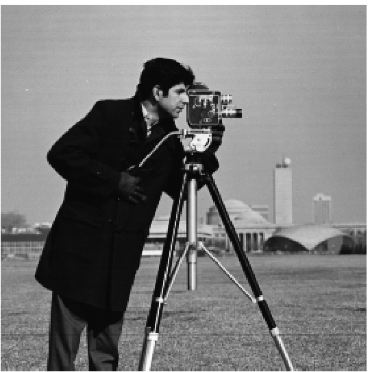
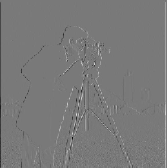
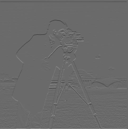
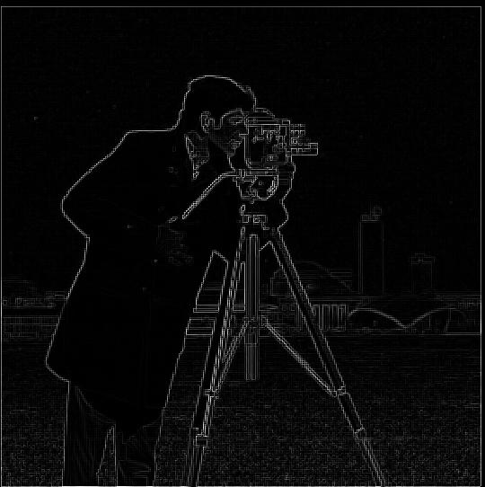
To start off this project, I used simple difference operators to compute the image gradients along the x and y axes for edge detection. By applying convolution with D_x = [[1, -1]] and D_y = [[1], [-1]] to the "Cameraman" image, I obtained the partial derivatives I_x and I_y , which highlight vertical and horizontal edges, respectively. 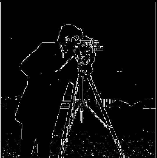I then combined these gradients to calculate the overall gradient magnitude, representing the strength of edges. The formula that I used for gradient magnitude was √ ((I_x)^2 + (I_y)^2). After testing different thresholds, I found that a value of 50 worked best for binarizing the gradient magnitude, producing a binary edge map that effectively highlights the detected edges in the image.

Original Image

X-gradient

Y-gradient

Magnitude of Gradient

Edges Detected

Derivative of Gaussian (DoG) Filter

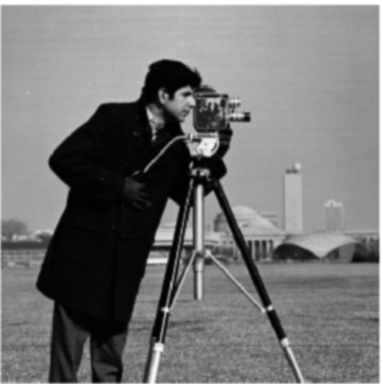
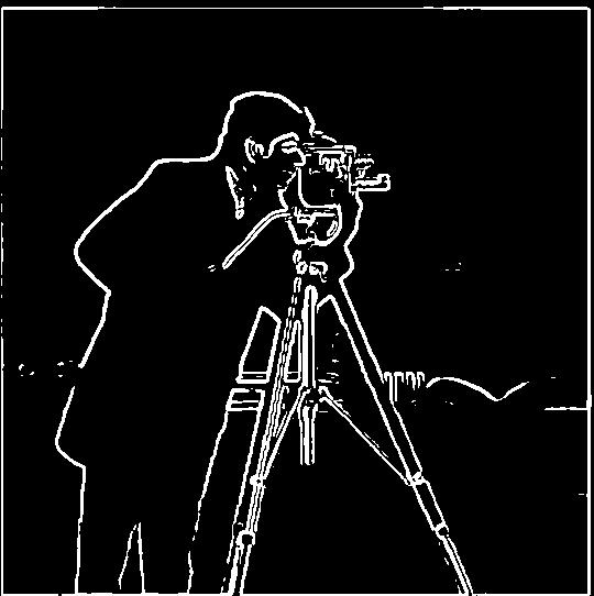
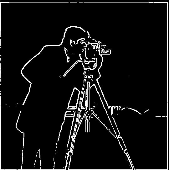
The Derivative of Gaussian (DoG) filter is an extension of the Gaussian blur, which smooths the image and computes the derivative. This is useful for detecting edges in the image after reducing noise. Below are the images of the cameraman with a blurr applied and then the edge detection. Also, there is a second method of calculating the derivative of guassian filters to only use one convolution per direction.

Cameraman Blurred

Binary Edge Image With Blurr

DoG Applied

After applying the blurr, we can see that there is a lot less noise which is extremely helpful for edge detection. Also, we know that by the properties of convolution, we can use the derivative of guassians to convolve and get the same answers. This is confirmed by the example above.

Image "Sharpening"

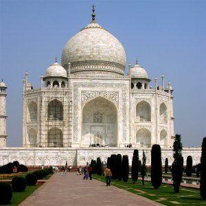
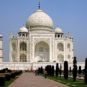
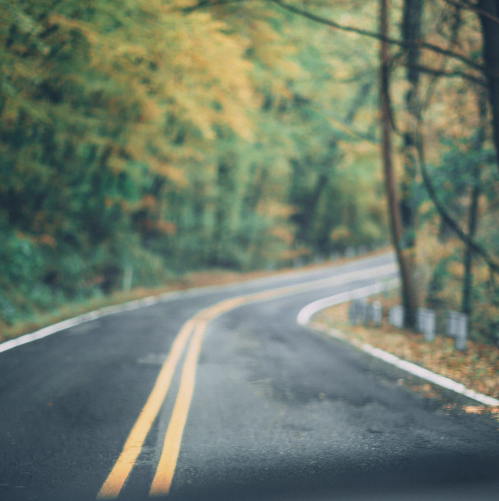
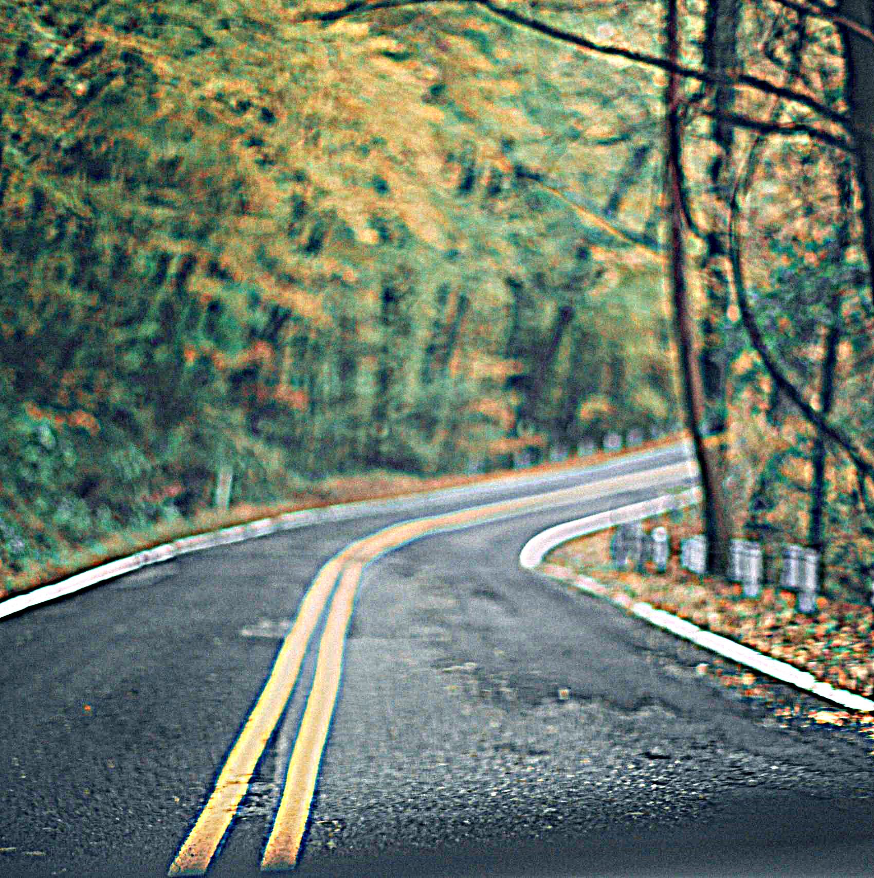
In this section, I implemented a function to enhance image details by isolating and amplifying high-frequency components. This was achieved by applying a Gaussian blur to the image, subtracting the blurred version to isolate the high frequencies, and adding them back to the original image, scaled by a factor α. For color images, each RGB channel was sharpened individually before recombining them. I tested this on the images of the Taj Mahal as well as a picture of a blurry road with trees. 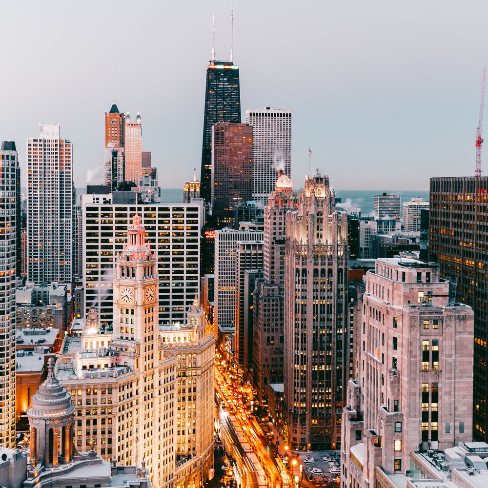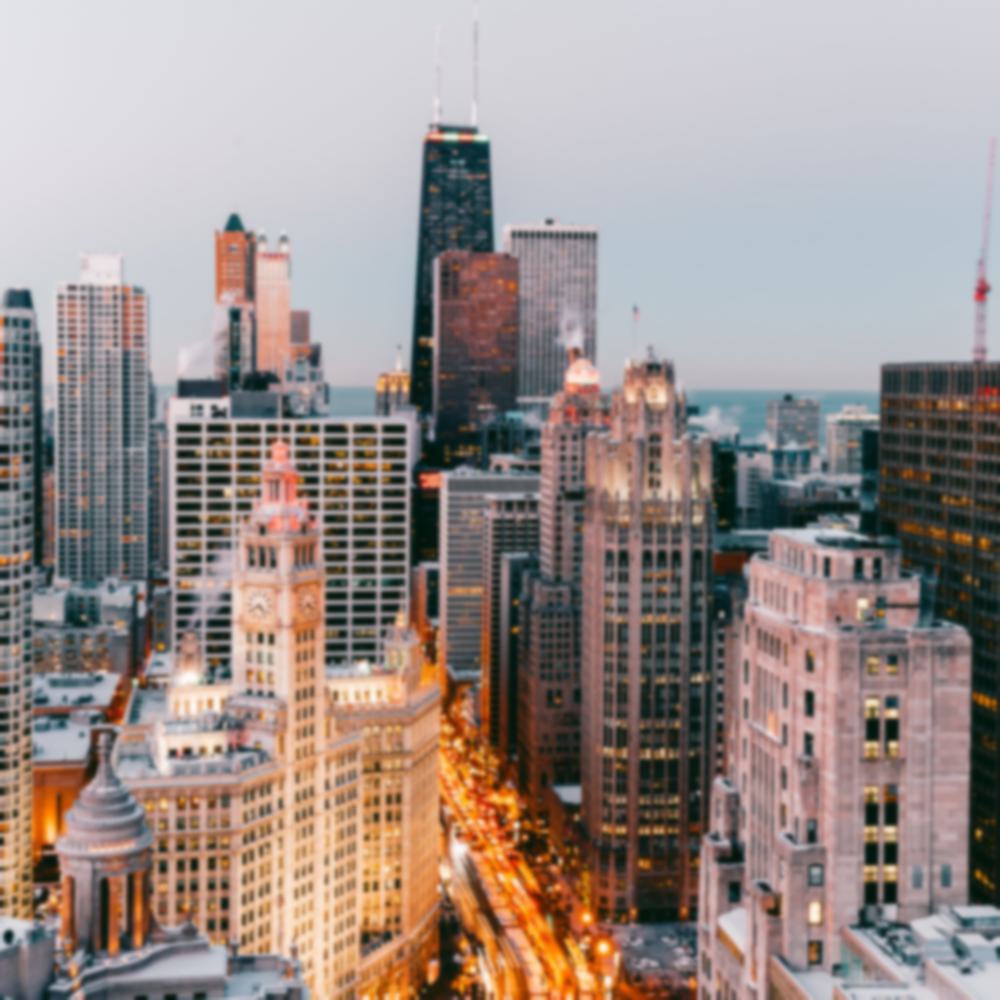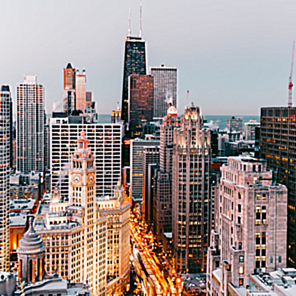I also confirmed it worked by taking a non-blurry image of a city, applying a blur and then sharpening it.

Original Taj Mahal

Taj Mahal Sharpened

Original Blurry Road

Blurry Road Sharpened

Original City

City Blurred

City Re-sharpened

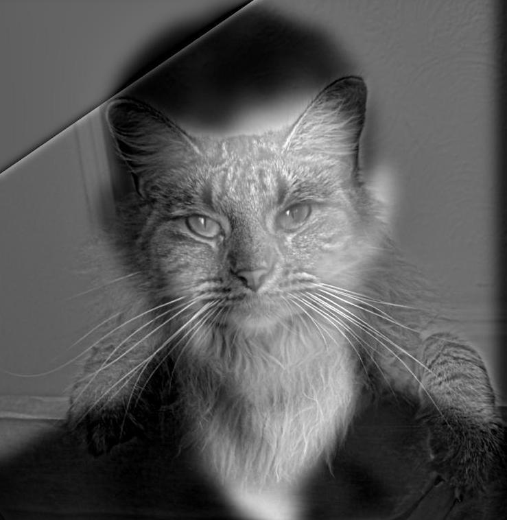
Hybrid Images

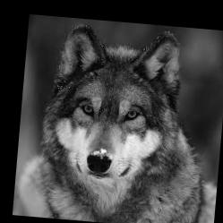
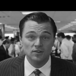
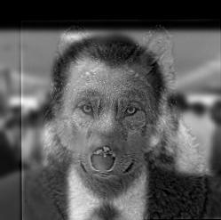
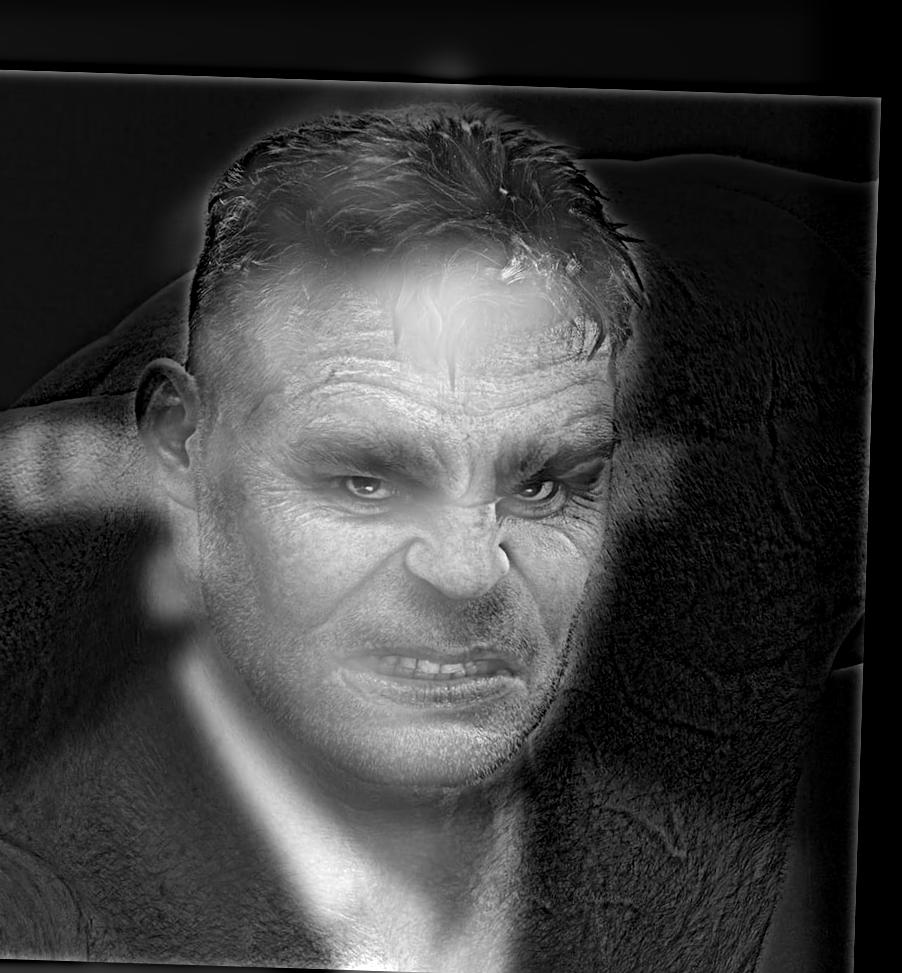
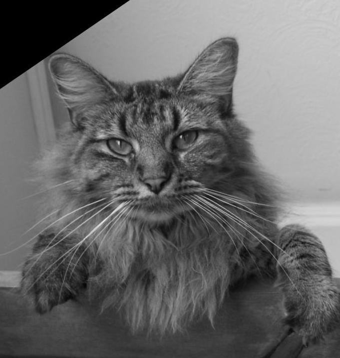
I created a hybrid image by combining the low-frequency components of one image with the high-frequency components of another. First, I applied a Gaussian blur to the first image ("Derek") to extract its low frequencies, and separately blurred the second image ("Nutmeg") to isolate the high-frequency details by subtracting its blurred version from the original. The hybrid image was then formed by adding the low-frequency content of the first image to the high-frequency content of the second, producing a result where the viewer sees one image up close and another from a distance. After aligning the two images using a provided function, I experimented with different blur levels to create the final hybrid image. This method blends the two images in a way that shifts perception based on viewing distance.

Aligned Gray Nutmeg

Aligned Gray Derek

Derek + Nutmeg

Aligned Gray Wolf

Aligned Gray Leonardo

Leonardo + Wolf

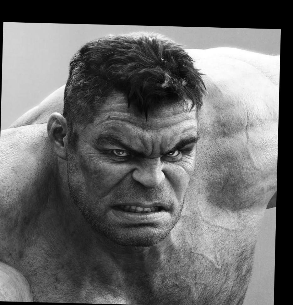
Aligned Gray Hulk

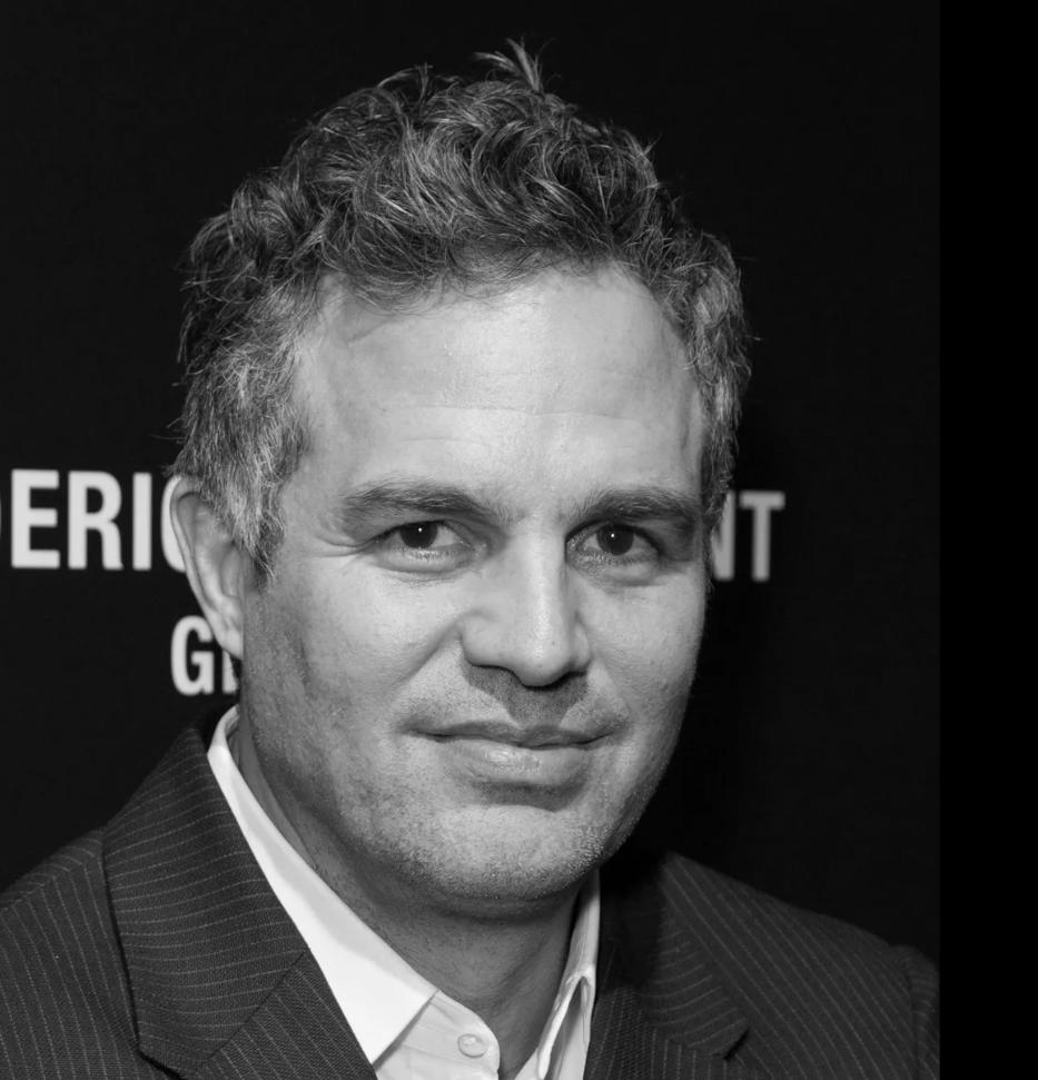
Aligned Gray Ruffalo

Ruffalo + Hulk

Fourier Analysis

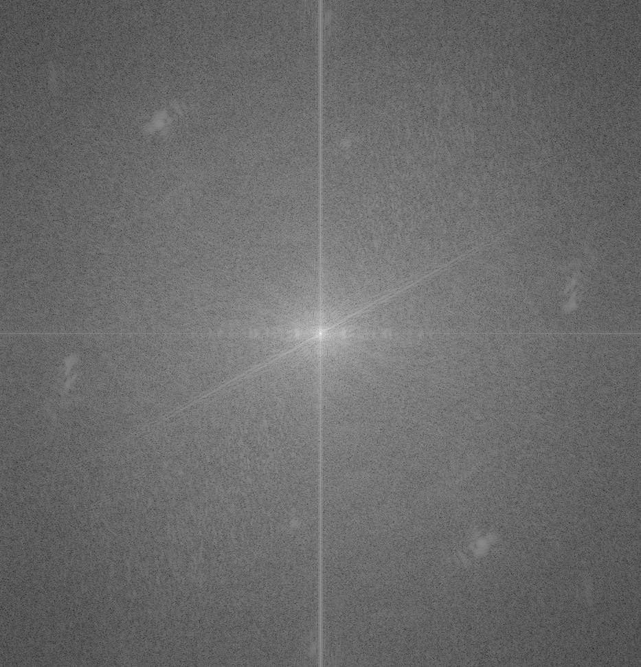
Next, I performed a Fourier Transform Analysis on images to visualize their frequency components and observe the effects of filtering. I first implemented a function to compute the 2D Fast Fourier Transform of an image using np.fft.fft2. The FFT converts the image from the spatial domain to the frequency domain, where each point represents a specific frequency. I then shifted the zero frequency component to the center of the spectrum using np.fft.fftshift and applied a logarithmic transformation to the magnitude to enhance the visibility of the frequencies for display purposes. 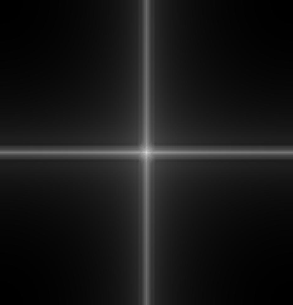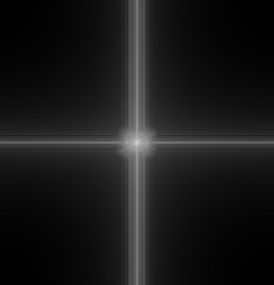Next, I applied this FFT analysis to the images of "Ruffalo" and "Hulk" to visualize their frequency content. 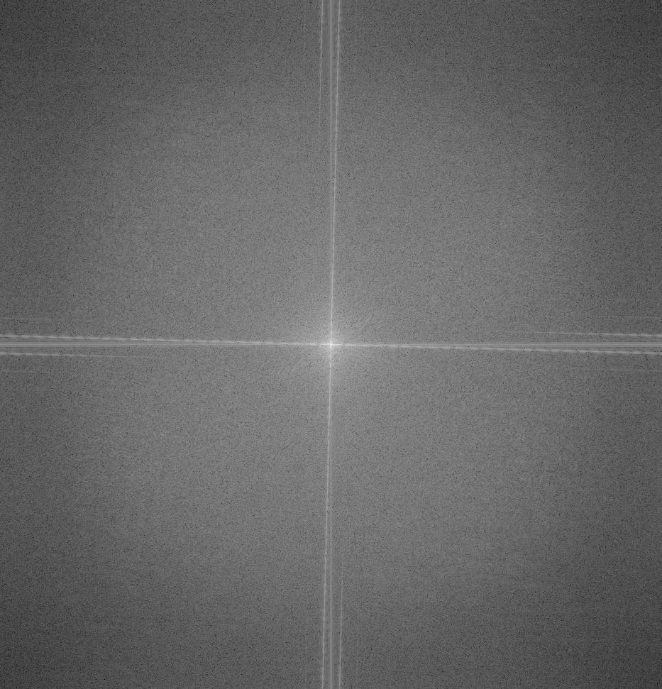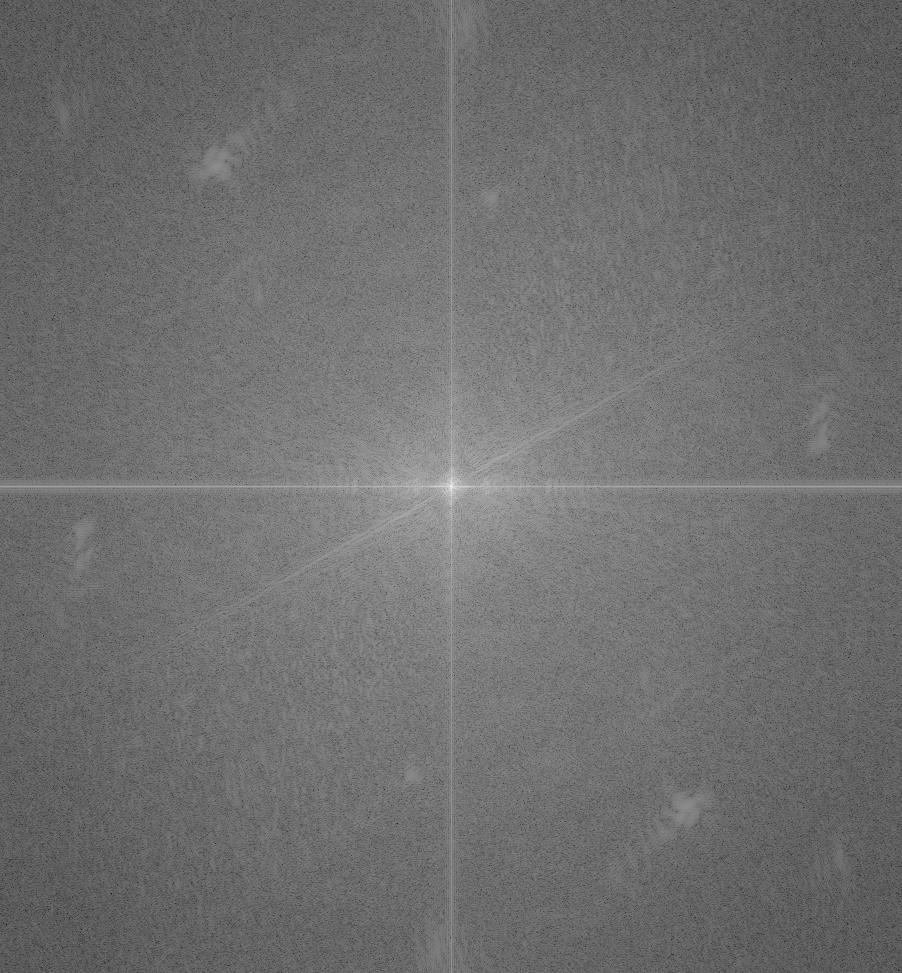After that, I used Gaussian filters to isolate the low-frequency components in both images, displayed their filtered frequency spectra, and subtracted the low frequencies from the "Ruffalo" image to obtain the high frequencies. Finally, I combined the low-frequency components of "Hulk" with the high-frequency components of "Ruffalo" to create a hybrid image, and I displayed its frequency spectrum. This Fourier analysis allowed me to explore how the combination of different frequency bands contributes to the resulting hybrid image, making the transitions between the two images more understandable in terms of their frequency characteristics.

Hulk FFT

Ruffalo FFT

Hulk Filtered FFT

Ruffalo Filtered FFT

Hybrid FFT

Gaussian and Laplacian Stacks

In this section, I generated and visualized Gaussian and Laplacian Stacks for multi-resolution analysis of images. The Gaussian stack was created by progressively blurring the image at each level using a Gaussian filter with an increasing sigma value, resulting in a series of images that become smoother at higher levels. The Laplacian stack was then formed by subtracting each blurred image from the next level in the Gaussian stack, isolating the high-frequency details between levels, with the final level representing the most blurred, low-frequency version of the image. I applied this process to two grayscale images, "Apple" and "Orange," creating five levels for each image. The Gaussian stack showed progressively blurred versions, while the Laplacian stack revealed finer details at each level. This multi-resolution decomposition is useful for analyzing and manipulating images across different scales and frequencies.

Orange Gaussian Stack

Orange Laplacian Stack

Apple Gaussian Stack

Apple Laplacian Stack

Multiresolution Blending

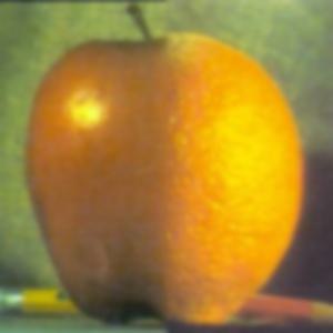
In this section, I implemented multiresolution blending using Gaussian and Laplacian stacks to seamlessly merge images based on different masks. First, I created three types of masks: vertical, horizontal, and circular, which define the blending regions in the images. The blending process works by constructing Gaussian and Laplacian stacks for each image and the mask. The Gaussian stack progressively blurs the images at multiple levels, while the Laplacian stack isolates the details between each level of the Gaussian stack, splitting the images into high and low-frequency components. To blend two images, I applied the Laplacian stacks of both images to their respective color channels (RGB) and used the Gaussian stack of the mask to smoothly combine the two Laplacian stacks. The blending is achieved by weighting each image based on the mask, creating a transition between the two images. Finally, I reconstructed the blended image by adding the frequency levels from the Laplacian stacks, producing the final composite. 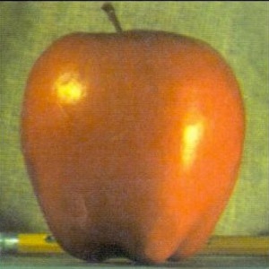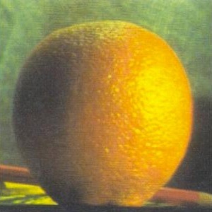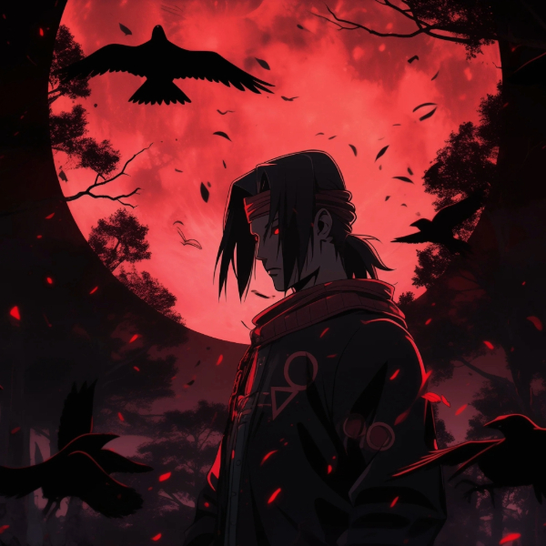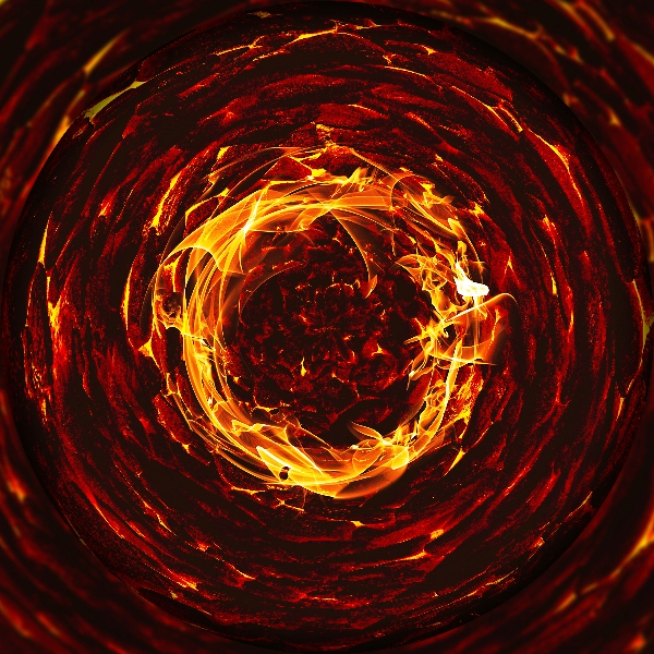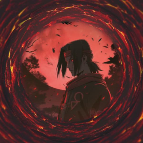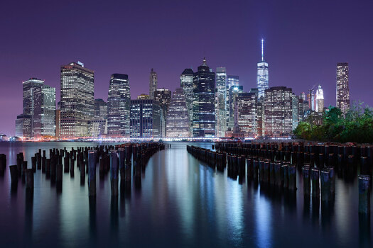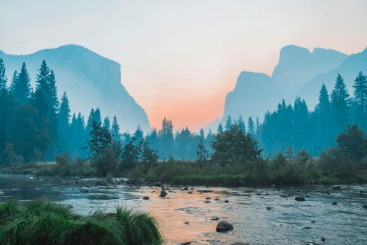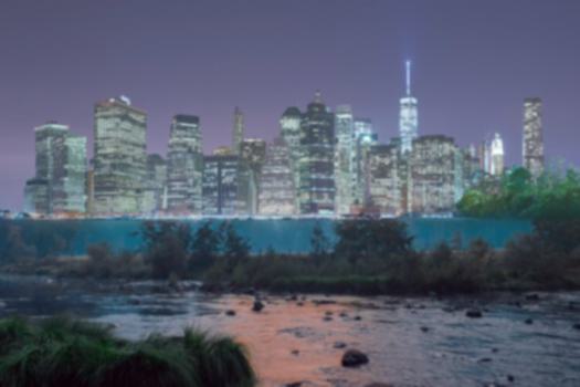I tested this approach on three image pairs: "Apple + Orange" using a vertical mask, "Night + River" using a horizontal mask, and "Itachi + Fire" using a circular mask.