CS 180 Project 4: Auto-stitching and Photo Mosaics
Homography, Image Warping, Feature Matching, and Auto-stitching
Jason Lee
Collecting Pictures
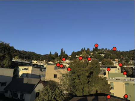
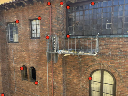
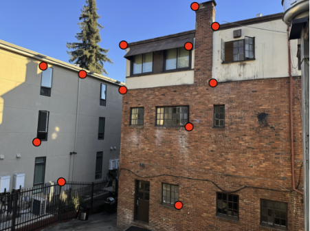
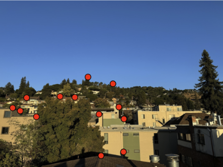
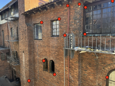
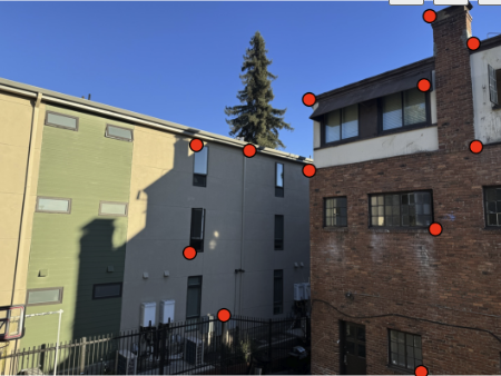
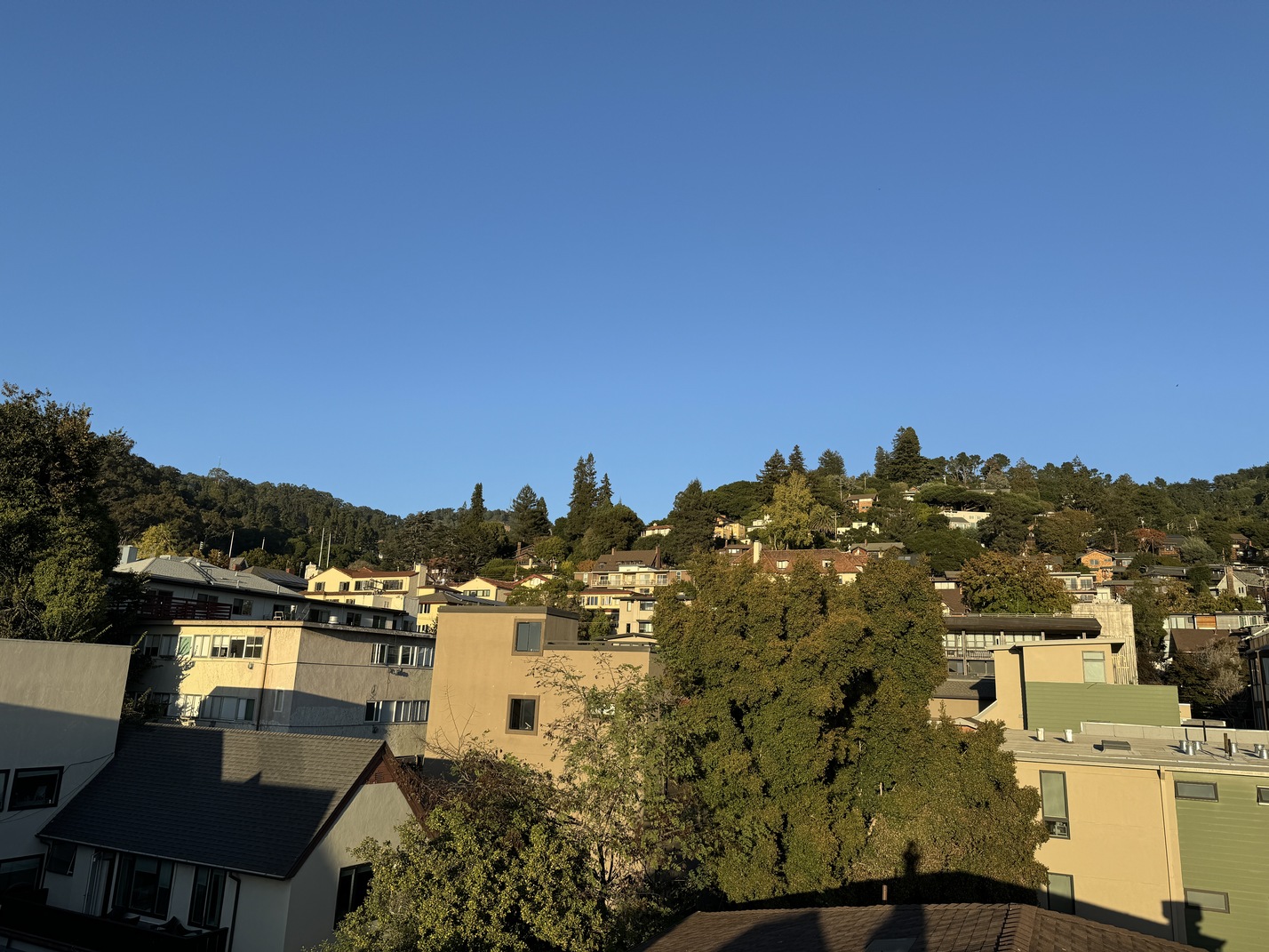
In the first stage of the project, I collected three sets of two pictures of Southside Berkeley
from slightly different perspectives. These images were chosen to capture enough
variation for the subsequent alignment process. To prepare for image warping, I
identified and defined 12 key correspondence points between the pairs of photos, ensuring
that important landmarks were consistently mapped across both images, which would
facilitate accurate homography recovery and seamless image blending later in the project.

Tree Left

Brick Left

Alley Left

Tree Right

Brick Right

Alley Right
Recover Homographies
To align the images, I needed to determine a homography matrix that allow me to transform the images. In this 3 by 3 matrix, the bottom right value
is 1 as a scaling factor. The homography can then be calculated by selecting corresponding points in both images and setting up a system of equations.
using corresponding homogenous points, we can derive two equations. By expanding and simplifying the terms, and then dividing by the homogeneous coordinate
we obtain two equations per point pair. Then all of the n pairs will result in 2n equations with 8 unknowns. As suggested by course staff, I used 12 pairs instead of
the minimum of four so that my images could alight more precisely. The equations are displayed below:

Homography Equations
Warping Images
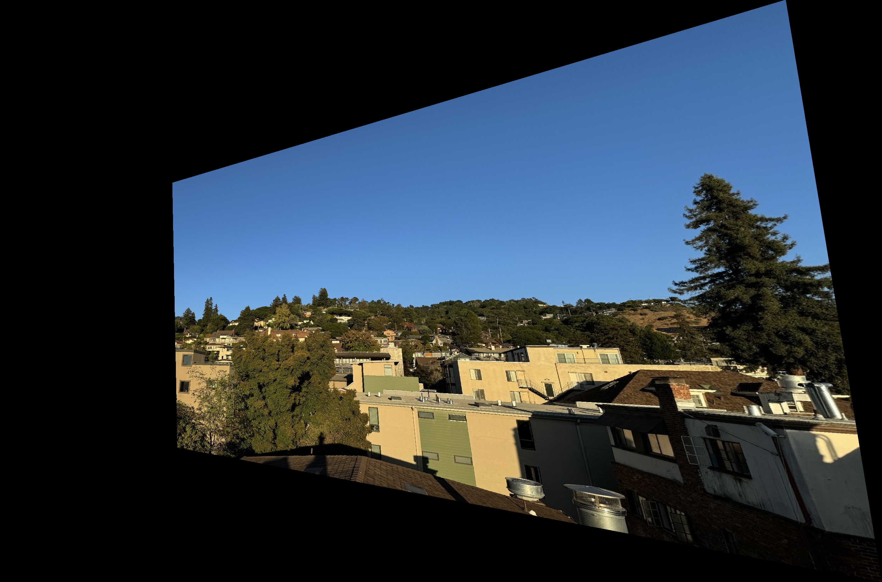
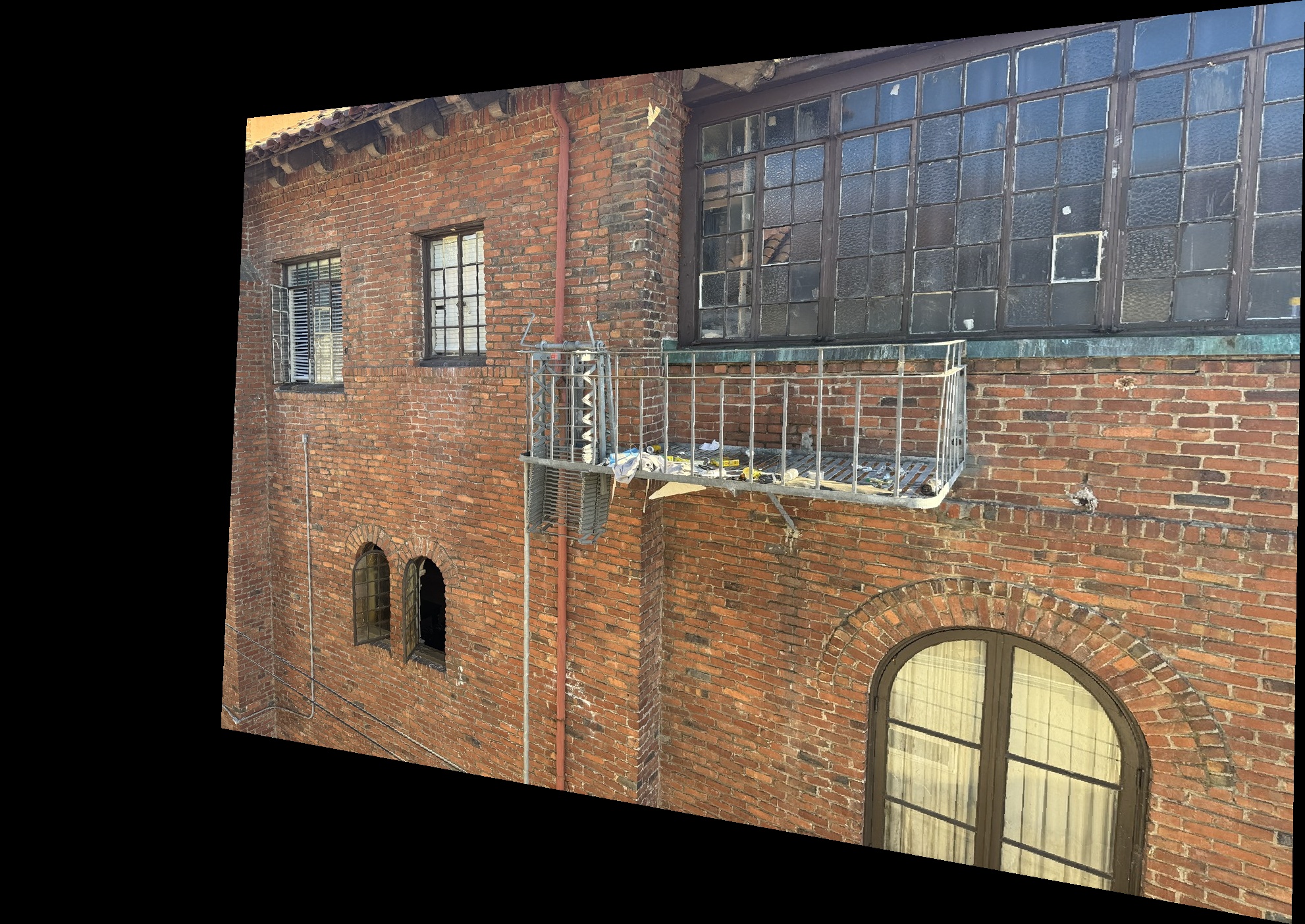
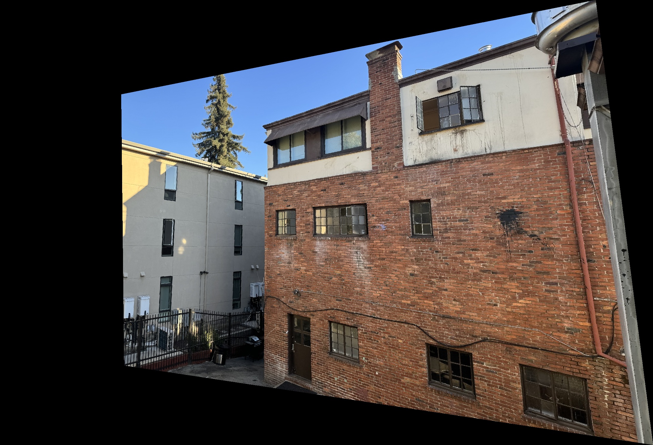
Next I implemented a function warpImage that applies a homography transformation to warp an image onto a new plane.
The function takes in an image, a homography matrix, and an output size for the resulting warped image. Inside the function,
I calculated the inverse of the homography matrix to map each pixel from the output image back to the original image
coordinates. For every pixel in the output, I used the inverse homography to find its corresponding position
in the original image, then sampled the pixel value from that position if it was within the bounds of the
original image. Moreover, I also added a box function so that I could properly calculate a box that would fit the comined image
of the left (base) and right (warped).

Tree Right

Brick Right

Alley Right

Tree Right Warped

Brick Right Warped

Alley Right Warped
Image Rectification
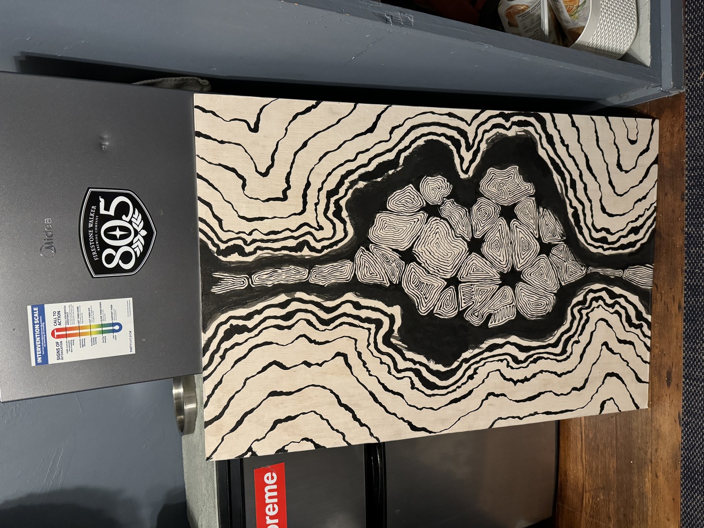
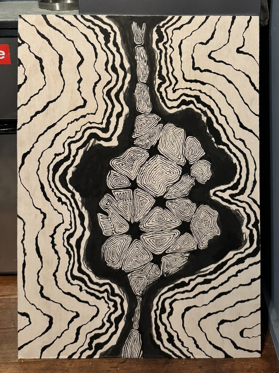
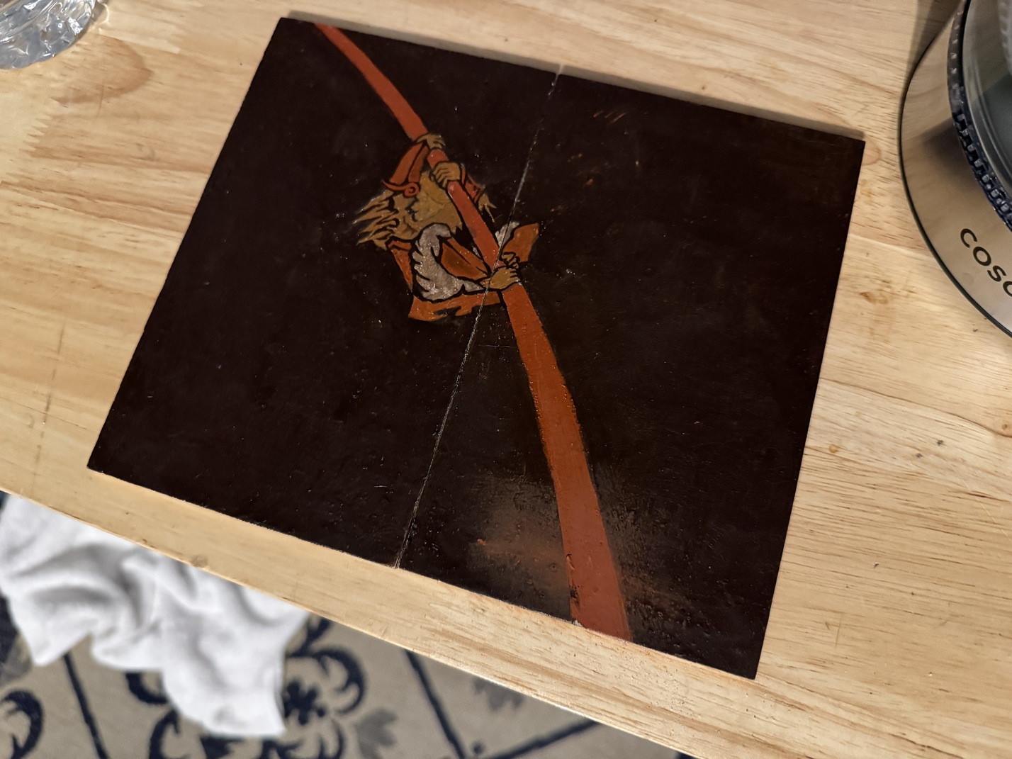
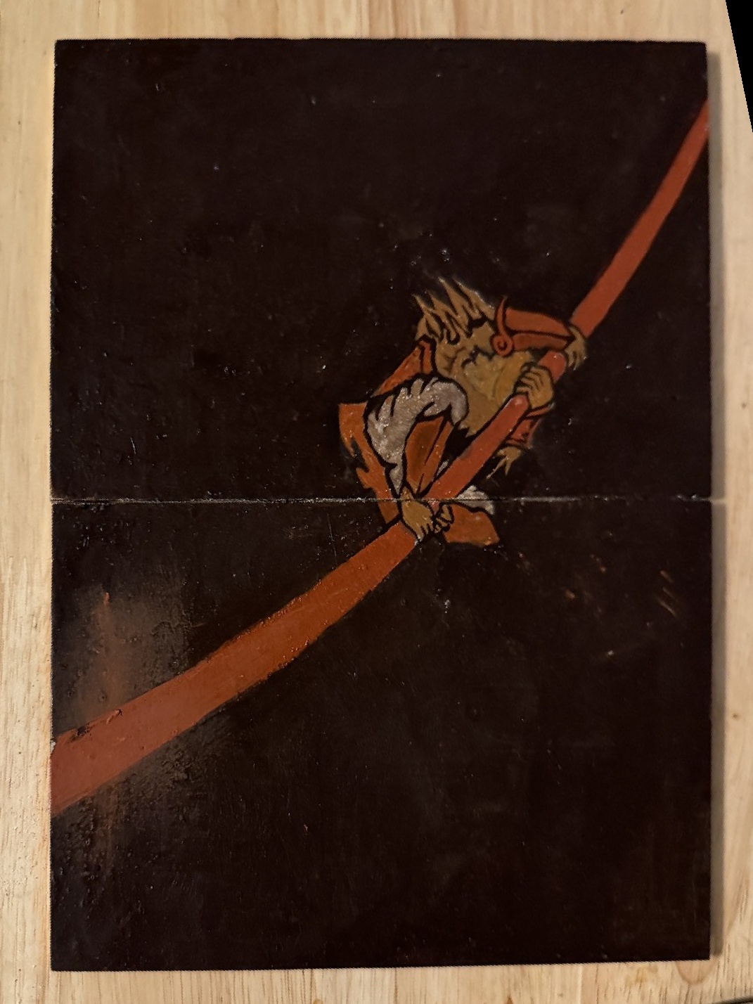
To test the homography and image warping functions, I took a skewed two pictures of paintings I recently completed and rectified it.
To do this, I chose the four corners of the painting and also using a blank image i chose the four corners as the set of points.
I then found the homography matrix and used it to warp the skewed painting to a rectangle.

Original Image

Rectified Image

Original Image

Rectified Image
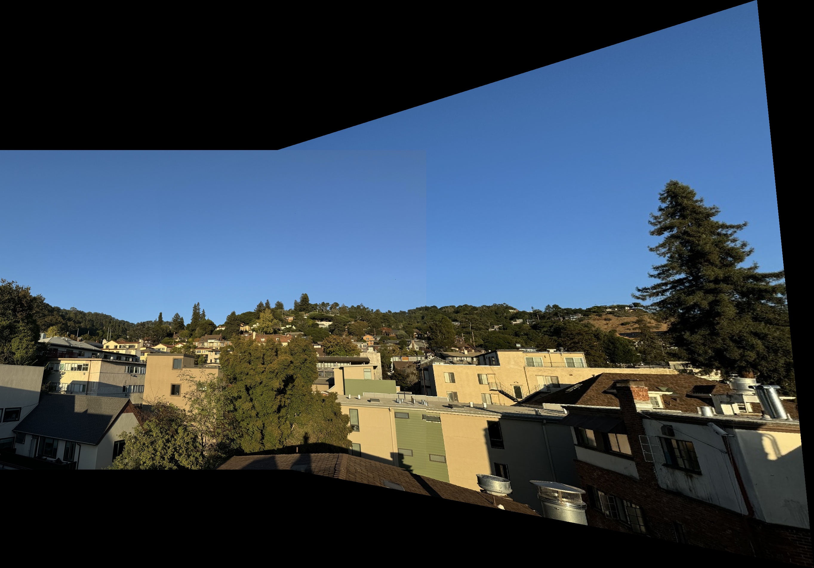
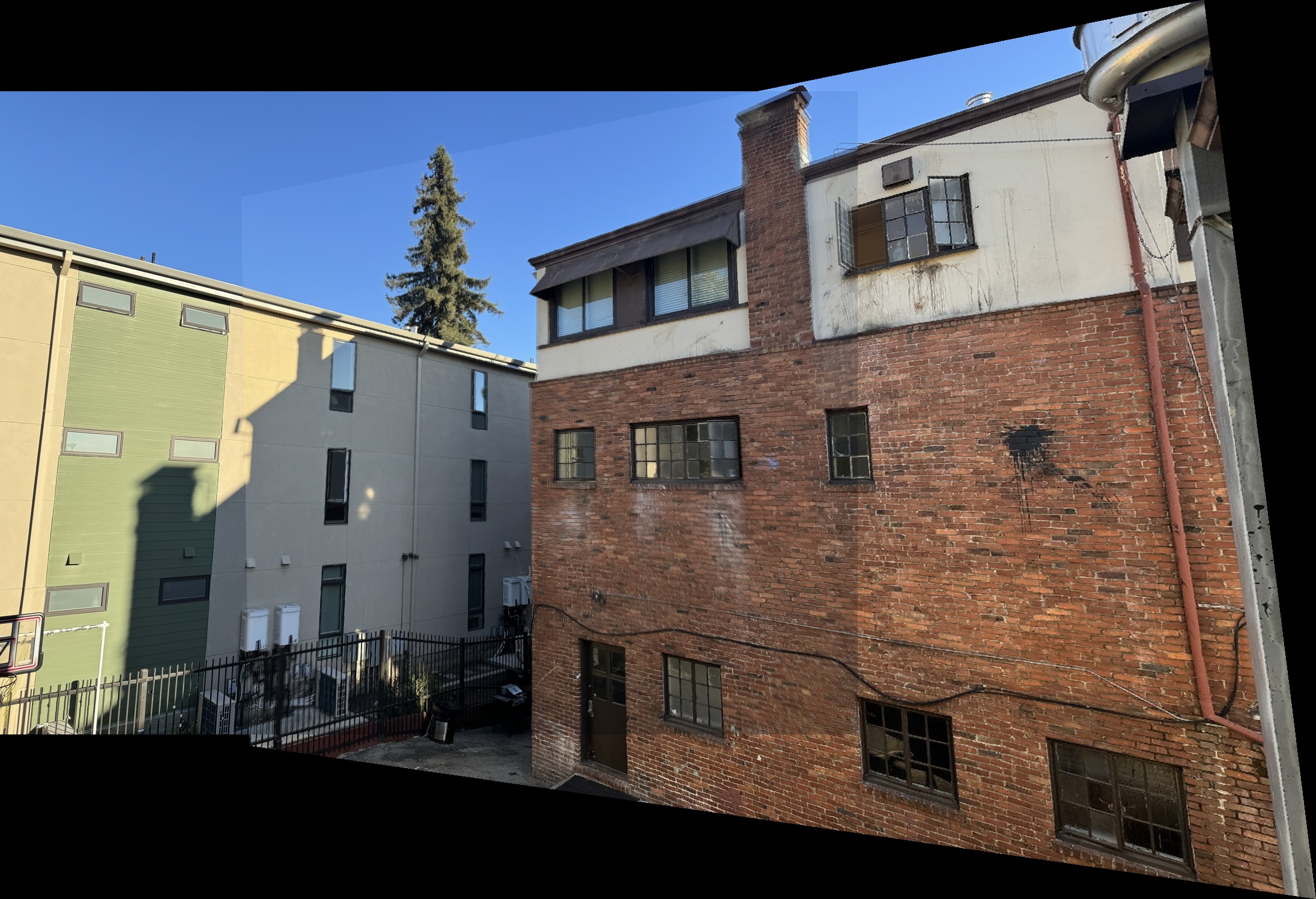
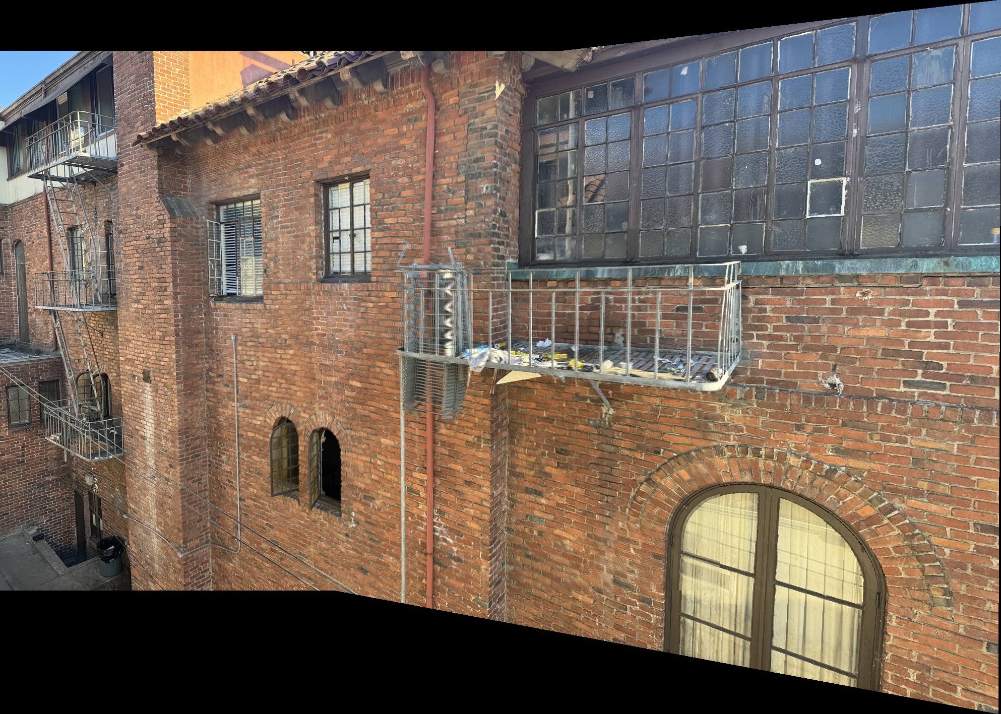
Blending Mosaic
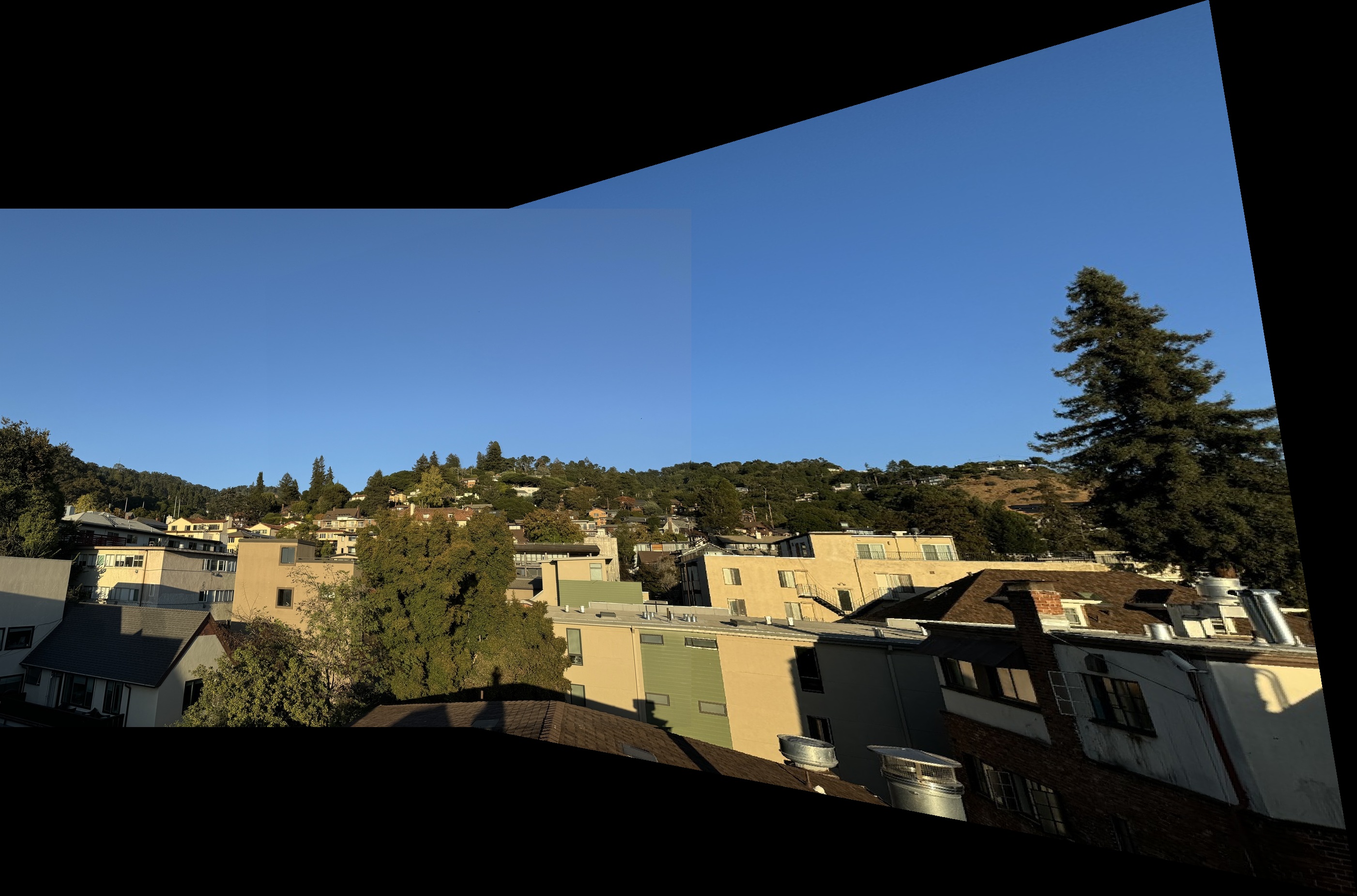
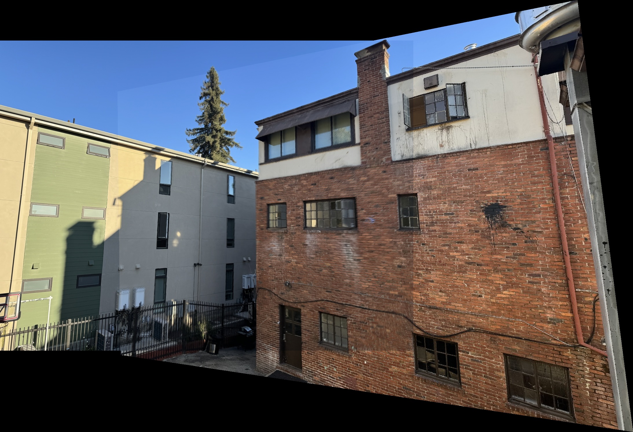
In the final section, I blended the warped right image with the left image to create a seamless mosaic.
First, I created binary masks for both images to identify the regions where they overlap.
I set the right image as the base and then applied a weighted average blending in the overlapping
areas. For non-overlapping regions, I tried playing with the weights of the averaging. I tested many alpha
values for each of the three comined images. It worked seemlessly for the first two. However, the third image
was hard to create a seamless transition due to the original nature of the images. One was a lot darker than the
other.

Trees Blended Mosaic

Brick Blended Mosaic

Alley Blended Mosaic
Detecting Corner Features
For the next part of the project, I aimed to have auto corner detection for image stitching.
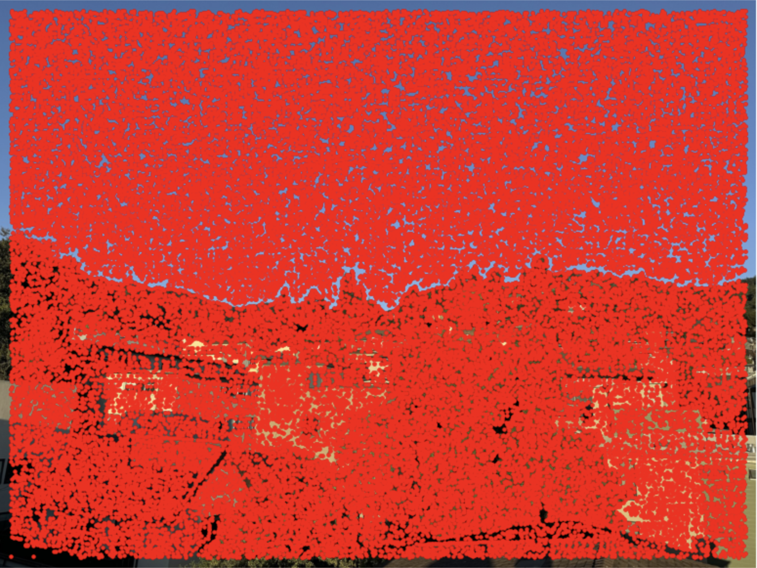
I applied corner detection using the Harris Corner Detection algorithm. This algorithm was given
in the project starter code. The effect of this code was to identify strong corner points
that would serve as features for matching across images. Here are the Harris corners found in the
Trees left image. As you can see, there are thousands of corners detected that span the entire image,

Original Image

Harris Corners
Adaptive Non-Maximal Suppression
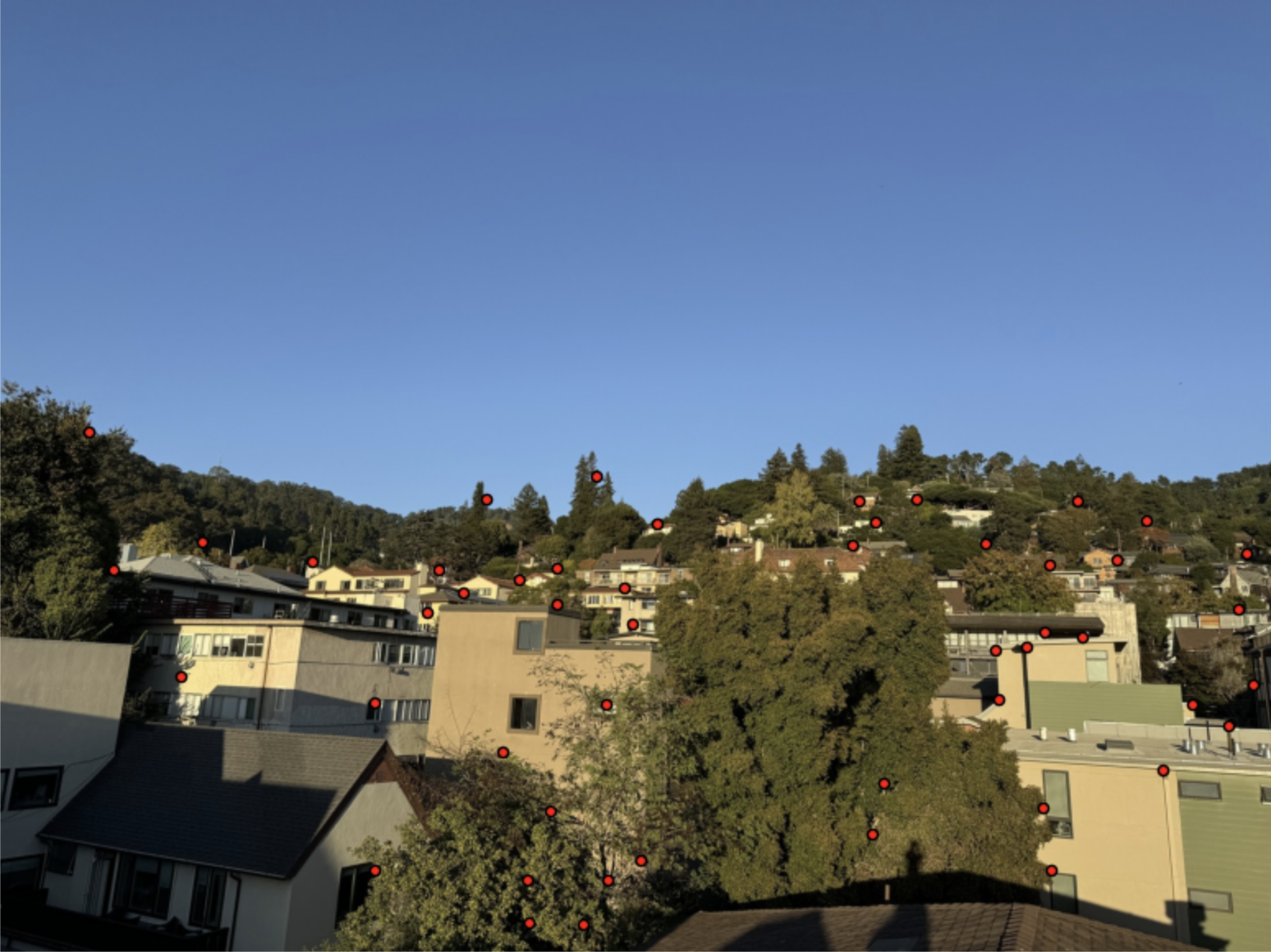
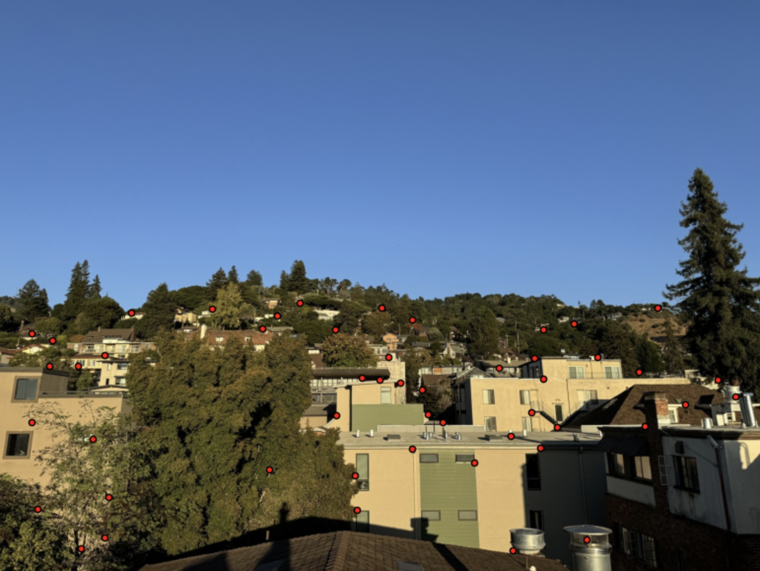
To reduce the number of corner points and focus on the most significant ones, I applied Adaptive Non-Maximal Suppression (ANMS).
The ANMS code I implemented aimed to select a spatially distributed subset of strong corner points for feature matching.
It does so by calculating a suppression radius for each corner point, representing the minimum distance to a
stronger neighboring point. Using a KD-Tree for efficient nearest-neighbor search, the compute_radius function finds
these distances, and I parrellelized this function across all points for efficiency. Finally, the points are sorted by
radius, and the top num_points are selected, yielding a set of well-separated, high-quality corners for robust feature extraction.

Trees Left ANMS

Trees Right ANMS
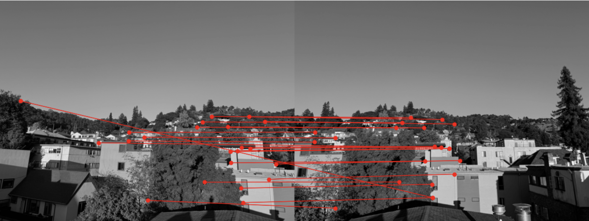
Feature Matching
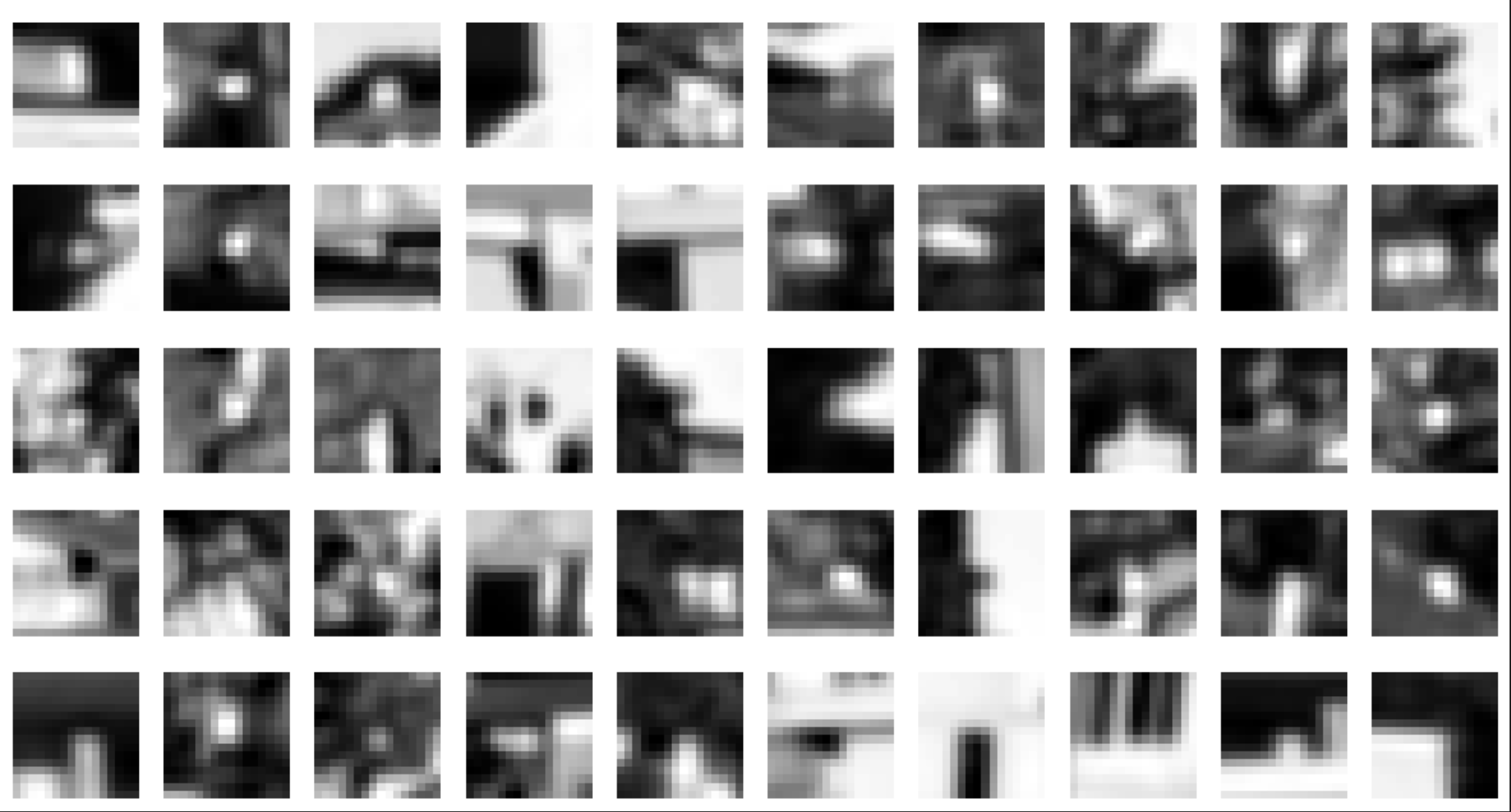
I then matched features between the images by comparing the feature descriptors. I matched features between two descriptor
sets by finding the two closest matches for each descriptor and applying Lowe's ratio test to ensure distinctiveness.
Only matches where the closest match is significantly better than the second-best are retained, resulting in high-quality
feature correspondences. However, notice how there are features that are matched incorrectly.

Feature Matching
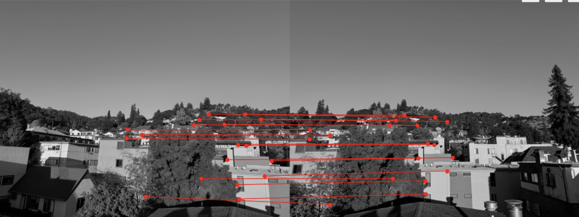
RANSAC
To improve the accuracy of feature matching, I applied the RANSAC algorithm, which iteratively selects random subsets of matches,
estimates a homography, and checks its consistency across all matches. This helps in filtering outliers and retaining only
the most reliable correspondences. After applying RANSAC, the points that were incorrectly matched are eliminated.

RANSAC Result
Final Results
Here are the final results using manually defined correspondence points versus the points found through corner detection. I think
that because I selected a good amount of points manually, the final resutls did not differ much. For the brick images, I think the over
lap is a little less blurry which means that auto detection is probably still more reliable.

Trees Manual Stitching

Alley Manual Stitching

Brick Manual Stitching

Trees Auto Stitching

Alley Auto Stitching

Brick Auto Stitching
What I Learned
In this project, I learned about the fundamentals of image processing, including feature extraction,
matching, homography, and RANSAC. The coolest part for me was learning how to extract and match
features between images, which feels incredibly powerful and versatile. I can see how this technique c
ould be applied in countless areas, from object detection to panorama creation. As an artist, this project
inspired me to explore creative applications of these techniques. I’m excited about the idea of creating
an art project that stitches together corner features from similar paintings or drawings. By aligning
and blending these images, I could produce a unique, mosaic-like piece that highlights patterns and
connections between my works in a way I hadn’t imagined before.
